Costly Financial Intermediation

Problem Setup

Consider a two-period economy with two types of households:

{\begin{matrix} Type A (fractionθ) : y_{0}^{A} ≫ y_{1}^{A} (rich today, poor tomorrow) \end{matrix}

{\begin{matrix} Type B (fraction1 - θ) : y_{1}^{B} ≫ y_{0}^{B} (poor today, rich tomorrow) \end{matrix}

Both maximize discounted log-utility:

U (C_{0}^{i}, C_{1}^{i}) = \log (C_{0}^{i}) + β \log (C_{1}^{i}), i \in {A, B} .

For some further mathematical intuition:

{max}_{C_{0}^{i}, C_{1}^{i}} & \log (C_{0}^{i}) + β \log (C_{1}^{i}) s.t. & C_{0}^{i} + \frac{1}{1 + r_{d}} C_{1}^{i} = y_{0}^{i} + \frac{1}{1 + r_{d}} y_{1}^{i}

Type A households naturally want to save (lend), while Type B want to borrow.
If financial markets were frictionless, a single equilibrium interest rate would perfectly match the supply of savings with the demand for borrowing.

The Reality: A Positive Spread

In practice, financial intermediaries impose a wedge between borrowing and lending rates:

r_{l} > r_{d}, (1 + r_{l}) = (1 + r_{d}) (1 + x), x \approx r_{l} - r_{d} .

The spread $x$ captures the inefficiency of intermediation:

Savers (Type A) earn the low deposit rate $r_{d}$ .
Borrowers (Type B) pay the high loan rate $r_{l}$ .

Individual Optimization

Type A (savers)

Optimal consumption solves:

C_{0}^{A} = \frac{y_{0}^{A} + \frac{1}{1 + r_{d}} y_{1}^{A}}{1 + β}, C_{1}^{A} = β (1 + r_{d}) C_{0}^{A} .

Type A saves positively: $S_{0}^{A} = y_{0}^{A} - C_{0}^{A} > 0$ .

Type B (borrowers)

Optimal consumption solves:

C_{0}^{B} = \frac{y_{0}^{B} + \frac{1}{1 + r_{l}} y_{1}^{B}}{1 + β}, C_{1}^{B} = β (1 + r_{l}) C_{0}^{B} .

Type B borrows at $t = 0$ : $S_{0}^{B} = y_{0}^{B} - C_{0}^{B} < 0$ .

Market-Clearing and Equilibrium Rates

Deriving bond market clearing delivers equilibrium deposit and loan rates:

𝒟^{b o n d} = \int_{0}^{θ} S_{0}^{A} d i = θ (y_{0}^{A} - \frac{y_{0}^{A} + \frac{1}{1 + r_{d}} y_{1}^{A}}{1 + β})

𝒮^{b o n d} = \int_{θ}^{1} S_{0}^{A} d i = (1 - θ) (y_{0}^{B} - \frac{y_{0}^{B} + \frac{1}{1 + r_{l}} y_{1}^{B}}{1 + β})

Letting $𝒮^{b o n d} = 𝒟^{b o n d}$ and solving for $r_{l}$ and $r_{d}$ , we obtain the optimal rates of lending and borrowing, denoted with a $*$ superscript:

r_{d}^{*} = \frac{θ y_{1}^{A} + \frac{1 - θ}{1 + x} y_{1}^{B}}{β (θ y_{0}^{A} + (1 - θ) y_{0}^{B})} - 1,

r_{l}^{*} = \frac{(1 + x) θ y_{1}^{A} + (1 - θ) y_{1}^{B}}{β (θ y_{0}^{A} + (1 - θ) y_{0}^{B})} - 1 .

In the ideal case ( $x = 0$ ), these rates coincide.
In reality ( $x > 0$ ), they diverge.

Aggregate Utility Comparison between a Zero Interest Rate Gap Economy and an Interest Rate Gap Economy

The utility of the economy at large can be written as:

U_{a g g r e g a t e} & = \int_{0}^{1} U (C_{0}^{i}, C_{1}^{i}) d i & = θ [\log (C_{0}^{A}) + β \log (C_{1}^{A})] + (1 - θ) [\log (C_{0}^{B}) + β \log (C_{1}^{B})]

Let xp denote a positive interest rate difference ( $r_{l} - r_{d} > 0$ ) and xz denote a zero interest rate gap ( $r_{l} - r_{d} = 0$ ).

Since $r_{d, x p}^{*} < r_{x p} < r_{l, x p}^{*}$ , we can plug these back into our optimal conditions and compare the values of optimal utility:

U_{A, x p} < U_{A, x z}, U_{B, x p} < U_{B, x z} .

Graphical Interpretation

Savers graph

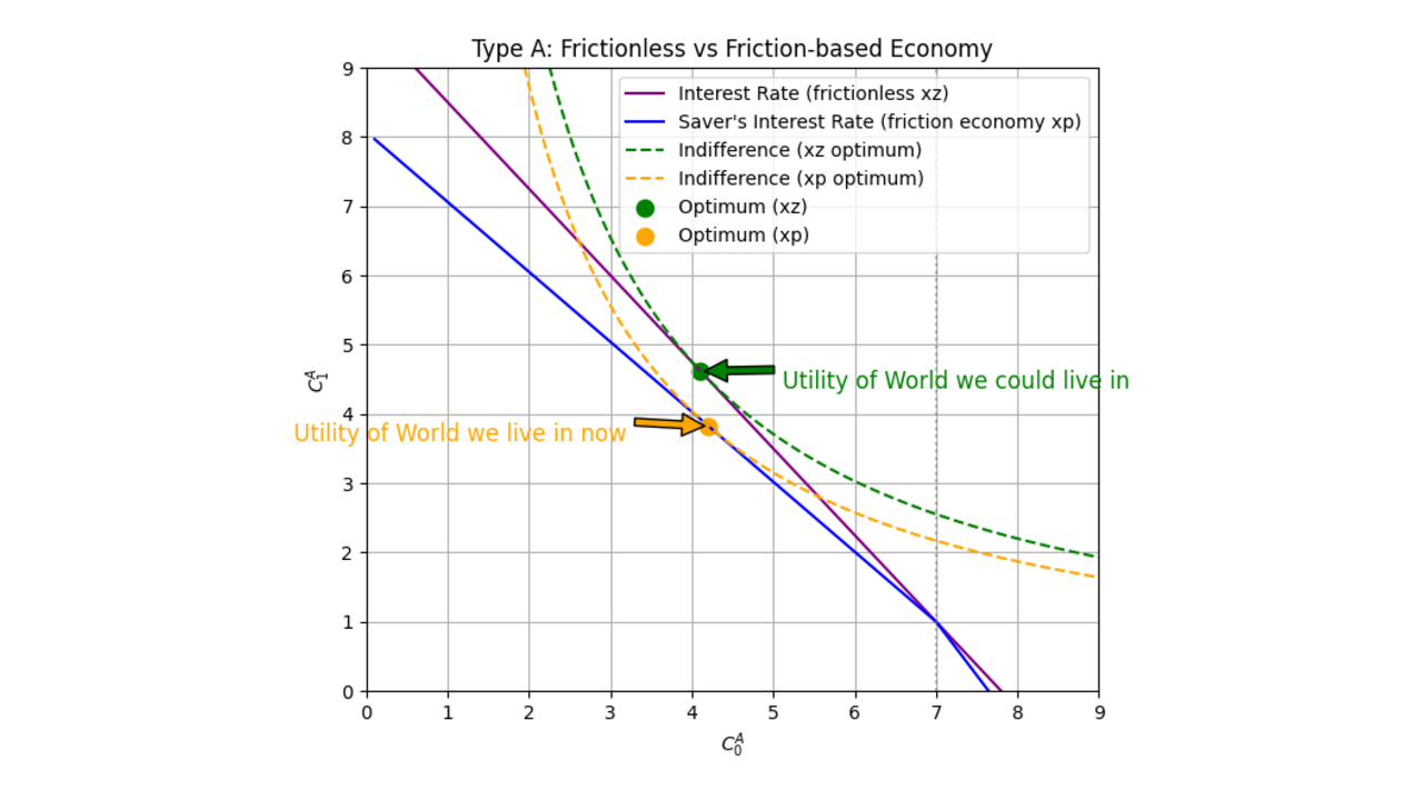
The blue and purple lines represent budget constraints as defined in the problem setup.
The blue line is a piecewise function that has a slope of $\frac{1}{1 + r_{d}}$ up until the point $(y_{0}, y_{1}) = (7, 1)$ .
Beyond that point, the slope changes to $\frac{1}{1 + r_{l}}$ .
The green and orange lines are indifference curves representing utility.

Borrowers graph

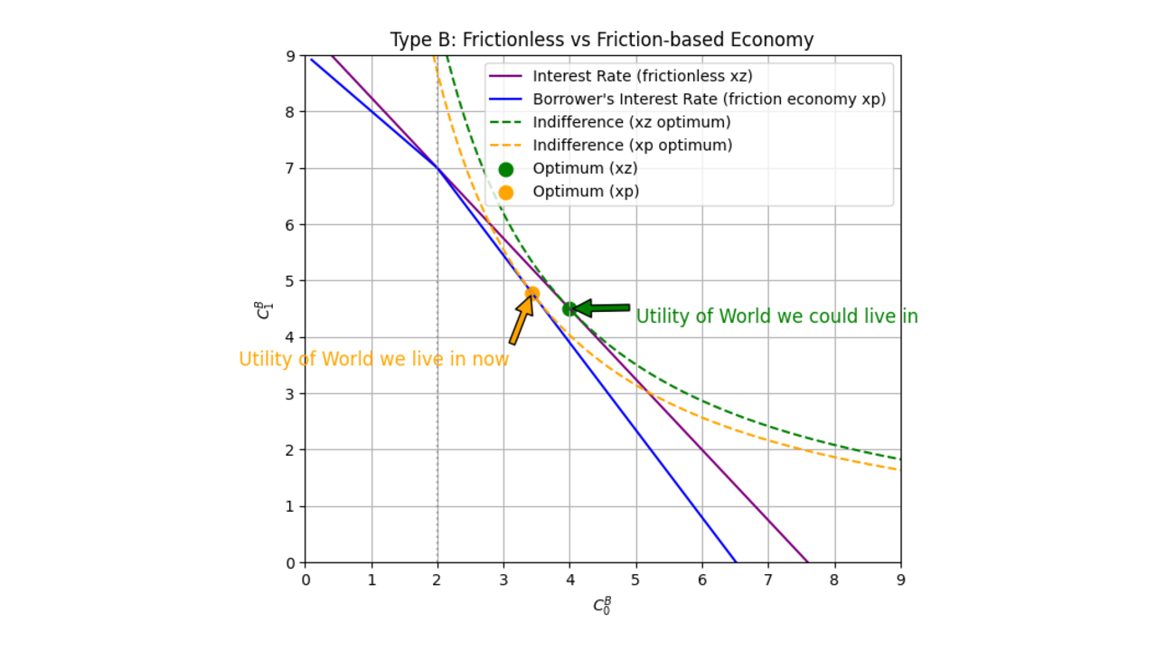
Similarly, the blue and purple lines represent budget constraints.
The blue line has a slope of $\frac{1}{1 + r_{d}}$ up to $(y_{0}, y_{1}) = (2, 7)$ , after which it changes to $\frac{1}{1 + r_{l}}$ .
The green and orange lines represent indifference curves.

Economic Interpretation

In the ideal frictionless economy, the interest rate is unique, and savings and borrowing are efficiently allocated.
In the real economy, intermediaries create a spread to pay for tellers, branches, credit analysts, etc.
Savers earn less, borrowers pay more, and society as a whole is worse off.

Moral:
We don’t live in the “ideal world” where credit flows at a single fair rate.
Instead, intermediation costs show up as a wedge between $r_{d}$ and $r_{l}$ , lowering utility for everyone who is borrowing or lending money.