Portfolio Optimization using a Reinforcement Learning based Iterative Solver – FGMRES

Link to research paper: Accelerated Portfolio Optimization And Option Pricing With Reinforcement Learning by Hadi Keramati and Samaneh Jazayeri: https://arxiv.org/pdf/2507.01972v1

Link to my code: https://github.com/Vekram1/ill_conditioned_ppo_RL_matrix_solver

Motivation

Something as trivial as solving x in Ax = b helps portfolio managers, economists, and traders execute optimized portfolios, test hypothesized financial models, and get real-time option pricing information. As one could imagine, solving for x has far-reaching uses in computer graphics, machine learning, fluid dynamics, and even traffic flow.

Just so we’re on the same page — when I write Ax = b, I don’t mean solving a single linear equation like 3x = 6. Instead, I am interested in solving a system of linear equations where:

A is an n × n matrix
b is an n × 1 vector
We solve for x, which has the same shape as b

Inverting A or using direct methods (like Gaussian elimination) gives precise results but is computationally expensive — especially as n gets large (imagine portfolios with thousands of assets).

Instead, we rely on iterative methods, which reduce the residual r = Ax – b over multiple steps.

Common iterative methods include the Jacobi method, Gauss-Seidel, and gradient descent.
This piece focuses on the Generalized Minimal Residual Method (GMRES) and its variant, Flexible GMRES (FGMRES).

Mean-Variance Portfolio Optimization Problem Setup

Below represents the constraint-based optimization that we are trying to solve:

{min}_{x} \frac{1}{2} x^{T} Σ x

s.t μ^{T} x = R_{t a r g e t}

e^{T} x = 1

We are trying to choose a vector x, representing our asset allocation, that minimizes the variance of the portfolio.

Σ is an n by n covariance matrix of asset returns. The expression ½ xᵀ Σ x represents the variance of the portfolio as a whole, and we would like to minimize that.

e is a vector of all ones, so the condition eᵀ x = 1 just means that the weights we assign to the assets in our portfolio must add up to 1.

μ is a vector of expected returns, so the condition μᵀ x = R_target says that the dot product of the expected returns with our chosen portfolio weights must equal our portfolio’s target return.

To solve this optimization problem, we usually use the Lagrangian method. I won’t go through all the steps here since they’re not so important in the big picture, but the result looks like a system of equations that we can write as A y = b, where:

A = | Σ  e   μ  |
    | eᵀ 0   0  |
    | μᵀ 0   0  |

y = | x |
    | λ₁|
    | λ₂|

b = |     0    |
    |     1    |
    | R_target |

In our portfolio optimization, using an iterative solver, our goal is to solve for y, which will also yield us our correct portfolio allocation x.

Understanding GMRES

Before diving into FGMRES, we need to understand GMRES — the foundation it builds upon.

Goal

We want to solve the linear system A x = b, where:

A is an m×m invertible matrix.
b ∈ Rᵐ, with ‖b‖ = 1 (for simplicity).

Step-by-Step Overview

1. Initial Guess and Residual

Start with an initial guess x₀ ≠ 0
Compute the initial residual:
r₀ = b – A x₀

2. Construct the Krylov Subspace

Iteratively build the Krylov subspace:

K_{n} (A, r_{0}) = span {r_{0}, A r_{0}, A^{2} r_{0}, \dots, A^{n - 1} r_{0}}

The solution lies in:

x_{n} \in x_{0} + K_{n}

3. Issue: Near Linear Dependence

The vectors {r₀, Ar₀, …, Aⁿ⁻¹r₀} can become nearly linearly dependent, degrading the subspace quality.

4. Solution: Arnoldi Process

The Arnoldi iteration constructs an orthonormal basis Qₙ = [q₁, q₂, …, qₙ] and an upper Hessenberg matrix Ĥₙ:

A Q_{n} = Q_{n + 1} {\tilde{H}}_{n}

5. Rewriting the Solution Form

Since xₙ ∈ x₀ + Kₙ:

x_{n} = x_{0} + Q_{n} y_{n}

Minimize residual ‖b – A xₙ‖, equivalent to:

{min}_{y_{n}} ‖ {\tilde{H}}_{n} y_{n} - β e_{1} ‖_{2}

Once solved for yₙ, substitute back into xₙ = x₀ + Qₙ yₙ to approximate the solution.

GMRES effectively reduces a large m×m system into smaller least squares problems of size (n+1)×n, where n ≪ m.

FGMRES – The Iterative Method Our RL Agent Will Use

FGMRES (Flexible GMRES) extends GMRES by allowing different preconditioners at each iteration.

What is a Preconditioner?

A preconditioner M is a matrix that approximates A but is easier to invert.
We solve M⁻¹A x = M⁻¹b, improving the conditioning of A and speeding convergence.

M = I → trivial, no improvement
M = A → perfect convergence, but as costly as solving A⁻¹ directly

The art lies in finding a cheap but effective M.

QR as a Preconditioner

Using QR decomposition, the system becomes:

Q ᵀ A x = Q ᵀ b \Rightarrow R x = Q ᵀ b

QR is robust to ill-conditioning and efficient on smaller blocks, though full QR of A is impractical.

GMRES with Preconditioning

Without preconditioning:

K_{n} (A, r_{0}) = span {r_{0}, A r_{0}, A^{2} r_{0}, \dots, A^{n - 1} r_{0}}

With preconditioning:

C : = M^{- 1} A, z_{0} : = M^{- 1} r_{0}

K_{n} (C, z_{0}) = span {z_{0}, C z_{0}, C^{2} z_{0}, \dots, C^{n - 1} z_{0}}

Pseudocode

In psuedocode, FGMRES looks like this:

Input: Matrix A ∈ R^(m×m), vector b ∈ R^m, restart parameter k
Output: Approximate solution x to A x = b

1. Choose initial guess x₀
2. r₀ = b – A x₀
3. β = ||r₀||
4. v₁ = r₀ / β
5. V = [v₁]                  # Orthonormal basis vectors
6. H = zeros((k+1, k))       # Upper Hessenberg matrix

7. For j = 1 to k:
       w = A vⱼ
       For i = 1 to j:        # Arnoldi orthogonalization
            hᵢⱼ = ⟨w, vᵢ⟩     # Take dot product
            w = w – hᵢⱼ vᵢ    # Orthonormalize against existing basis
       End
       hⱼ₊₁,ⱼ = ||w||         
       vⱼ₊₁ = w / hⱼ₊₁,ⱼ
       Append vⱼ₊₁ to V

8. Solve the least squares problem:
       minimize || β e₁ – H y ||
   for y ∈ R^k

9. Compute solution update:
       x = x₀ + V y

Instead, if we apply a preconditioner, the Arnoldi process builds this Krylov subspace as such, where C and z_0 are:

\[C : = M^{- 1} A, z_{0} : = M^{- 1} r_{0} \] \[K_{n} (C, z_{0}) = span {z_{0}, C z_{0}, C^{2} z_{0}, \dots, C^{n - 1} z_{0}} \]

The pseudocode version looks like:

Input: Matrix A ∈ R^(m×m), preconditioner M (invertible), vector b ∈ R^m, restart parameter k
Output: Approximate solution x to A x = b

1. Choose initial guess x₀
2. r₀ = b – A x₀
3. z₀ = M⁻¹ r₀
4. β = ||z₀||
5. v₁ = z₀ / β
6. V = [v₁]                  # Orthonormal basis vectors
7. H = zeros((k+1, k))       # Upper Hessenberg matrix

8. For j = 1 to k:
       w = A vⱼ
       w = M⁻¹ w             # Apply preconditioner to our Krylov space
       For i = 1 … j:        # Arnoldi orthogonalization
            hᵢⱼ = ⟨w, vᵢ⟩
            w = w – hᵢⱼ vᵢ
       End
       hⱼ₊₁,ⱼ = ||w||
       vⱼ₊₁ = w / hⱼ₊₁,ⱼ
       Append vⱼ₊₁ to V

9. Solve the least squares problem:
       minimize || β e₁ – H y ||
   for y ∈ R^k

10. Compute solution update:
       x = x₀ + V y

FGMRES Preconditioning

With FGMRES, we can let the preconditioner change at every iteration. This is helpful for us, since we will be using block preconditioning (i.e., we precondition matrix A on different block sizes).

How preconditioning is set up in OUR PROBLEM

Because A is sparse, we can improve convergence of the iterative solver by splitting the matrix A into smaller block sizes of size l × l.

So what we end up having is:

M = diag(A₁, A₂, …, Aₖ) where each block Aᵢ ∈ R^(l × l).

The last block just takes whatever is left over.

Example: if A is an 11×11 matrix, and our chosen block size is 5, then M will be composed of:

M = A_{1 : 5, 1 : 5}, A_{6 : 10, 6 : 10}, A_{11, 11}

At each inner iteration j of FGMRES, the current preconditioner Mⱼ⁻¹ is applied by solving each block (via QR in our case). What makes this “flexible” is not just that the blocks can be different sizes; it’s that the preconditioner itself can change from one iteration to the next. In our setup, that flexibility shows up because the block size (and thus the block structure of Mⱼ) is chosen adaptively at each step. What we end up seeing is that:

v_{j + 1} \propto A M_{j}^{- 1} v_{j}

and

C_{j} = A M_{j}^{- 1}

in our Krylov subspace. Once we compute the next candidate vector vⱼ₊₁, we orthonormalize it against the previous basis vectors. This process gives us the Krylov subspace we build the approximation from.

The main idea here is that block preconditioning reduces the number of iterations needed to reach a good solution x. With GMRES (fixed block size), the preconditioner is the same at every step. With FGMRES (flexible block size), we adapt the block size at each iteration, which can lead to faster convergence on tough problems.

RL Training

This was the fun part of the project. While the math going behind iterative solvers was a little painful for me to learn, creating the environment for the agent, training the agent, adjusting rewards, and testing the agent on different problems was quite fun and very satisfying. I used the Stable Baseline3 (SB3) library for environment setup and learning. * Environemnt setup I will just focus on the fundamentals here which are the agent’s action and observation space. * Action Space * The action space of the agent was 8 discrete values. The paper never explicitly states what the action should be. The only thing that the author’s wrote was this: “In the PPO-based solver, the block size is limited to the set of integer values considered for the constant block size method, ensuring a fair comparison.” * I decided to use block sizes that were a small share of A. * Here I show the action space selection

def get_block_size(action, n: int) -> int:
    action = int(np.squeeze(action))
    """
    Map discrete action (0–7) to a block size that adapts with matrix size n.

    - Small n → minimum block size floor
    - Medium n → grow slowly with sqrt(n)
    - Large n → capped to avoid huge factorization cost
    """

    # Define scaling factors relative to sqrt(n)
    factors = [0.25, 0.35, 0.5, 0.7, 1.0, 1.5, 2.0, 3.0]

    # Compute baseline block size
    base_size = int(factors[action] * np.sqrt(n))

    # Enforce reasonable bounds
    block_size = max(4, base_size)       # minimum useful size
    block_size = min(block_size, 128)    # hard cap to keep runtime reasonable

    return block_size

Observation Space
- My observation space was a little more off script from the research paper. The authors had the observation space strictly as the residual norm. I believed that I could achieve further optimization of the agent in testing by defining an observation space that was comprised of a 4-dimensional continuous vector. The four features of the observation space are
  1. Relative Residual Norm: This is the ratio of the current residual norm to the initial residual norm. A value closer to 0 indicates better convergence.
  2. Log of the residual norm: The logarithm of the relative residual norm, provides better scaling for tracking improvements when the residual gets very small which it absolutely can and did in my testing.
  3. Normalized Matrix Size: The logarithm of the matrix size (n) normalized by a maximum size. This is essential for the agent to generalize across different problem sizes.
  4. Normalized Current Iteration: The current iteration divided by the maximum number of iterations. This tell the agent how far along the solver is in its run and can make decisions accordingly

# Define observation space: 4 continuous features
# This gives the agent more context for generalization.
# [0]: Relative residual norm (norm_k / norm_0)
# [1]: Log of the relative residual norm
# [2]: Matrix size normalized by log scale (log(n) / log(max_n_seen_in_training))
# [3]: Current iteration number normalized
self.observation_space = spaces.Box(
    low=np.array([0.0, -np.inf, 0.0, 0.0], dtype=np.float32),
    high=np.array([1.0, 0.0,  np.inf, 1.0], dtype=np.float32),
    shape=(4,),
    dtype=np.float32
)

Action Selection To understand how the agent behaves, we have to understand the algorithm it follows, the reward function it is given, and how this all impacts what action the agent picks.
- Algorithm - Proximity Policy Optimization (PPO)
- PPO is the specific RL algorithm used to train the agent. The main goal of PPO is to find an optimal policy (i.e a mapping from observations to actions) by iteratively updating the policy. It does this by collecting data from the environment and using that data to improve the policy. This algorithm is relatively simple to implement and performs comparably or better that state-of-the-art approaches
  - Proximal Policy Optimization (PPO), which perform comparably or better than state-of-the-art approaches while being much simpler to implement and tune.
- Reward Function
  - The reward function is defined within my FGMRESEnv class. I have is where python reward = (prev_residual_norm - curr_residual_norm) / prev_residual_norm The goal is to encourage the agent to chooses actions (block sizes) that lead to a significant reduction in the system’s residual norm at each step. A positive reward means the residual norm decreased, while a negative reward means it increased. The agent is trained to maximize the cumulative reward over an entire episode, which means its goal is to find a sequence of block sizes that leads to the fastest and most stable convergence.

Results of Testing

Finally, we have reached the results of this experiment. Would my results match the ones the researchers in the “Accelerated Portfolio Optimization and Option Pricing with Reinforcement Learning” paper got?

There wasn’t a lot of information on what datasets the ppo agent was supposed to be trained on. I did know that for their testing, they used datasets from the old University of Florida Sparse Matrix Collection, which is now managed under Texas A and M university Sparse Matrix Tamu. So I decided to pick a group of 7 sparse matrices to train on, specifically

TRAIN_MATRICES = [
("Newman", "polbooks"),
("Grund", "meg1"),
("Newman", "polblogs"),
("Grund", "b_dyn"),
("Marini", "eurqsa"),
("Hollinger", "g7jac010sc"),
("Grund", "poli_large")
]

where TRAIN_MATRICES[i] = ${\ < G r o u p, \ < N a m e}$ from the dataset. I thought this would be good enough for training. My test matrices were from the group Grund. The matrices were the poli and poli3 matrices. Here were the results of my data. I have included the number of iterations, time, and final residual for both my PPO agent solver and a fixed block size solver (the blocks were of size 500).

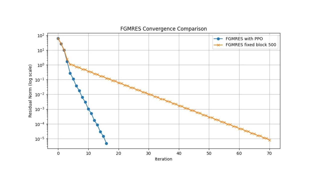
Poli 
FGMRES with PPO time: 1.80 seconds 
FGMRES iterations: 17 
FGMRES final residual norm: 4.82e-06 
FGMRES fixed block time: 52.85 seconds 
FGMRES fixed block iterations: 71 
FGMRES fixed block final residual norm: 7.94e-06

Poli graph

Poli3
FGMRES with PPO time: 143.58 seconds
FGMRES iterations: 19 FGMRES final residual norm: 7.01e-06
FGMRES fixed block time: 183.86 seconds
FGMRES fixed block iterations: 19 
FGMRES fixed block final residual norm: 7.01e-06

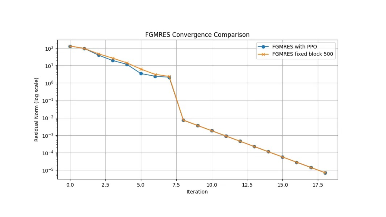Poli3 graph As you can see, the agent performed quite a lot better in terms of time and iterations on the poli dataset but performed marginally better in poli3. This disturbed me for quite a while, and actually led me to make many changes to training and the reward system. While the PPO agent in both instances outperforms the fixed block size preconditioner in terms of time, the number of iterations is quite high in poli3.

Ending Notes

My results were not what I had expected. I wanted to see the PPO agent crush the fixed sized block preconditioner, and it did in one of 2 of my cases. The research paper I read showed that the PPO agent far outperformed the fixed block size preconditioner in Poli3 as well. Regardless of my results, this was a great learning experience for me. I learned about GMRES, FGMRES, and how to train an RL agent. Thank you for reading. I hope you got something out of it.